LLM Inference TCO for Engineers: Price Request Shapes This Quarter

Inference cost title card illustration

The TCO of LLM inference is driven mainly by accelerators plus facility power and cooling, and by how requests are shaped, so fix request shape and utilization first. Token-normalized cost can mislead because a fixed inference-window energy cost hides what a request really consumes. Instrument per-request and per-token energy, then prioritize batching, caching and throughput gains before you change capital spending.

TL;DR:

Track request energy, token energy, time to first token, output speed, queue time, and GPU allocation time; token averages can hide rising energy per request.

Increase batch size only until output latency or key value memory becomes limiting; caching pays off mainly when prompts or retrieved documents repeat.

Benchmark candidate accelerators on decode throughput, memory bandwidth, cache capacity, and rack power using real traffic, because peak performance may poorly predict cost per request.

Compare owned capacity with cloud pricing across utilization, facility efficiency, and electricity rates; sustained demand favors ownership, while spiky low use favors rental.

Run a 30 to 90 day pilot, changing one optimization at a time and replaying identical production traces before making a major capital commitment.

What goes into an LLM inference TCO model?
Why are tokens not the full story for inference cost?
How do hardware choices change inference TCO?
Which optimization levers pay off most?
When does on-prem beat cloud on inference cost?
What checklist can your team run this quarter?
What does a TCO evaluation timeline look like from day one to steady state?
What cost ranges should you budget for each component?
How do security and compliance requirements change the TCO?
What do retraining, updates and lifecycle management add?
How do network topology and data locality affect on-prem inference cost?
Which vendor and licensing questions matter in private deployments?
Where do teams go wrong, and what should they do first?
How can we help you lower your LLM inference TCO?
FAQ
Sources

What goes into an LLM inference TCO model?

A usable spreadsheet has several buckets, and each one moves with utilization.

Hardware capex: GPUs or other accelerators, host servers, networking and storage, amortized over a realistic service life, based on your finance team’s planning assumptions.
Facility and infrastructure: power usage effectiveness (PUE), rack power density, cooling systems and the oversubscription limits your power feed allows.
Energy: electricity tied to GPU allocation, warmup and active time. Per-token energy falls as utilization rises, so idle capacity is the quiet cost.
Staff and operations: MLOps, monitoring, observability, incident response and the labor of swapping models.
Software and runtime: inference frameworks and any licensing, which change how much work each GPU-hour delivers.

The point of the map is that no bucket stands alone. A cheaper accelerator with weak decode throughput raises the energy, facility and staffing cost per delivered request. If you want a deeper treatment of the measurement side, our piece on tracking joules per token on prem covers instrumentation in detail.

Why are tokens not the full story for inference cost?

Every request splits into a prefill phase, which processes the prompt in parallel, and a decode phase, which generates output one token at a time. Request shape is defined by the model (M), hardware platform (P), batch size (B), context length © and output length (N). Two requests with the same token count can cost very different amounts of energy if their shapes differ.

This is where token-normalized metrics break down. Research on request and token energy costs shows that joules per token can fall simply because a fixed inference-window energy cost is spread across more tokens, even when total request energy rises. A dashboard that celebrates a falling J/token may be hiding a more expensive request.

Collect these metrics from production traces:

Request energy (Ereq) and token energy (Etoken)
Time to first token (TTFT) and time per output token (TPOT)
Queue time and GPU allocation time

Without Ereq and allocation time, you cannot tell true savings from amortization. Guessing at token shapes is the most common reason teams misattribute cost.

How do hardware choices change inference TCO?

Peak FLOPS is a poor purchasing guide. The datacenter TCO analysis on arXiv finds that theoretical peak performance often predicts cost-effectiveness badly, while performance on the thin GEMMs that dominate the decode phase is a stronger determinant, especially with lower-precision formats. A related FP8 TCO inquiry comparing accelerators such as the H100 and Gaudi 2 shows that precision and workload characteristics shift throughput ratios and therefore TCO.

When you evaluate a device, test these factors on your own traffic:

Decode throughput: measure thin GEMM and GEMV behavior at your real batch sizes, not vendor peak figures.
Memory bandwidth and KV cache capacity: these cap how large a batch you can hold and how long a sequence you can serve efficiently.
TDP and rack density: a hotter device changes cooling needs and how many accelerators fit in a power envelope, which feeds directly into facility cost.
Oversubscription headroom: better thermal behavior lets you pack more capacity into the same feed.

A device that wins on a spec sheet but starves on memory bandwidth during decode will cost more per request than a modest one that stays busy.

Which optimization levers pay off most?

Rank these by how cheaply you can try them, then measure Ereq before and after.

Batching: raise batch size until TPOT or KV memory becomes the constraint. Measure throughput per GPU-hour, and watch KV cache growth, which limits how far you can push.
Input and KV caching: high-similarity workloads, such as repeated system prompts or document-grounded Q&A, can see very large savings. Low-similarity traffic sees little.
Model sizing and specialization: comparisons of multi-purpose and task-specific models find general-purpose generative models can be orders of magnitude more expensive per inference for some tasks. If a small specialized model clears your quality bar, it is a major TCO lever.
Reduced precision: FP8 can raise throughput where validated, but it needs accuracy testing on your tasks. Our guide to LLM quantization and reproducible shipping covers the validation workflow.
Runtime improvements: FlashAttention, grouped query attention and speculative decoding reduce TTFT, TPOT or GPU active time.

Pro Tip: Change one lever at a time and replay the same production trace, so any drop in Ereq is attributable to a single change.

For a consultant’s view on operational playbooks, this guide to cutting GenAI inference costs frames a 90-day optimization sequence.

When does on-prem beat cloud on inference cost?

The breakeven model is simple. On the owned side, sum amortized capex, facility cost and operations per unit time. On the cloud side, take hourly or per-token pricing, adjusted for any committed-use discounts. The crossover is the utilization level at which the owned cost per delivered request drops below the rental cost.

Signals that tilt toward on-prem:

Sustained high utilization across the day
Data sovereignty or regulatory constraints
Predictable latency requirements
Unfavorable cloud power or cooling economics for your region

Signals that tilt toward cloud:

Spiky or seasonal workloads
Low average utilization
A desire to avoid operations overhead

Sensitivity matters more than the point estimate. Rerun the model across utilization, PUE and electricity rate ranges. Our overview of a gateway-first on-prem LLM for regulated enterprises shows how sovereignty requirements often settle the question before cost does.

What checklist can your team run this quarter?

This sequence maps to pilot work an engineering team can plan and complete.

Instrument production traces to derive B, C, N, Ereq and Etoken, using our notes on low-overhead LLM observability if tracing cost is a concern.
Run microbenchmarks on candidate hardware for decode throughput and KV cache behavior.
Compute the breakeven and its sensitivity to utilization, PUE and electricity rates.
Apply low-friction optimizations first, namely caching and batching, and measure real Ereq reductions.
If the numbers support it, plan a capacity pilot for on-prem deployment with thermal and power-aware scheduling.

Each step produces a number you can defend, which is the goal. A pilot that ends with a measured Ereq and utilization curve beats a vendor quote every time.

What does a TCO evaluation timeline look like from day one to steady state?

Think of the evaluation as phases, each ending in a decision.

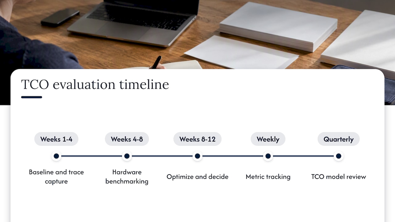
Four phases of an inference TCO evaluation

Weeks 1 to 4, baseline. Capture traces, derive request shape and record Ereq, TTFT and TPOT on whatever you run today. Without this baseline, every later saving is anecdotal. Build the first TCO spreadsheet from the five buckets above and mark every cell you had to guess.

Weeks 4 to 8, benchmark. Run decode-focused microbenchmarks on candidate hardware and a few model sizes. Validate any precision change against your accuracy tests. Replace guessed cells with measured ones.

Weeks 8 to 12, optimize and decide. Apply caching and batching, replay traces, and compute the breakeven against cloud pricing. At the end of this phase you choose: stay in the cloud, commit to on-prem capacity, or run a hybrid.

Ongoing operation. Treat TCO as a living metric. Track utilization, Ereq and queue times weekly, and review the model quarterly as traffic mix, model versions and electricity prices shift. Our TEVV roadmap for sovereign deployment lays out operational readiness steps that fit this cadence.

The failure mode is stopping after the decision. Utilization drifts, new models arrive with different request shapes, and a TCO that was once right can later be wrong. Scheduled re-measurement is cheap insurance against that drift.

What cost ranges should you budget for each component?

We do not quote market price ranges here, because current hardware, power and labor prices vary by region and change quickly, and a stale figure would mislead your budget. Use a worked example with inputs you replace instead.

Say you buy a server and amortize its cost over its service life while it runs at an average utilization. The annual amortized capex depends on the purchase price and service life. If utilization rises while the same traffic is served by fewer servers, capex per request falls, as can facility and staff costs per request. That is why utilization, not sticker price, dominates the arithmetic.

To fill in your own ranges, gather:

Hardware: vendor quotes for accelerators, servers, networking and storage, divided by planned service life.
Facility: your colocation or datacenter rate per kilowatt, multiplied by PUE.
Energy: measured kilowatt-hours per request from your Ereq data, multiplied by your local electricity rate.
Staff: fully loaded cost of the share of MLOps and on-call time the service consumes.
Software: licensing and support quotes for your runtime and orchestration stack.

The economics-of-inference research describes a production frontier with an optimal cost-effectiveness zone and diminishing returns beyond it, which is a useful reminder: past a certain scale, more capacity does not keep lowering unit cost. Budget for the zone, not the extreme.

How do security and compliance requirements change the TCO?

Private and air-gapped deployments trade cloud convenience for control, and the cost shows up in specific places. Air-gapped environments cannot pull container images, model weights or patches from the internet, so every update flows through a controlled transfer process with scanning and approval. That adds labor to each release and lengthens the path from a new model version to production.

Compliance also changes the bill of materials. Expect additional spend on:

Isolated infrastructure: dedicated networks, hardened hosts and physical access controls.
Audit and logging: tamper-evident logs, retention and review workflows, which consume storage and staff time.
Validation: testing, evaluation, verification and validation steps before a model goes live, repeated for each change.
Redundancy: you cannot burst to a public cloud during an outage, so failover capacity must live inside the perimeter.

These costs rarely appear in a cloud-versus-on-prem comparison built from hourly rates alone. They belong in the model as explicit lines, and they often decide the outcome because the alternative, sending sensitive data to a third party, may simply not be permitted. We build deployments inside customer-controlled infrastructure so the security posture is designed in rather than bolted on.

What do retraining, updates and lifecycle management add?

Models are not purchased once. New base models, fine-tunes, prompt changes and safety patches arrive continuously, and each one carries a cost: evaluation compute, regression testing, staged rollout and rollback readiness.

Lifecycle costs deserve their own lines:

Retraining and fine-tuning: GPU time and data preparation each time you adapt a model. Specialization pays back when it lets you serve a smaller model, so count the one-time training cost against the recurring inference savings.
Model swaps: replacing a model changes request shape, so batch sizes, cache hit rates and capacity plans need re-measuring. A swap is a mini TCO evaluation.
Decommissioning and versioning: keeping old versions available for reproducibility consumes storage and sometimes serving capacity.

Reproducibility is the discipline that keeps these costs bounded. If you can rebuild any shipped model artifact from recorded inputs, rollbacks are cheap and audits are straightforward. Build a release calendar, budget evaluation compute as a recurring operating line rather than a surprise, and re-run your Ereq baseline after every material change.

How do network topology and data locality affect on-prem inference cost?

Within a server, the interconnect between GPUs matters when a model is sharded across devices, because decode steps synchronize frequently. A topology with insufficient bandwidth between accelerators leaves them waiting, which lowers utilization and quietly raises cost per request.

Beyond the server, locality shapes both latency and spend:

Retrieval-heavy workloads: if documents live in a storage tier far from the GPUs, TTFT grows and accelerators idle during fetches. Keeping indexes and document stores close to compute cuts that stall.
Cross-site traffic: moving prompts, embeddings or KV state between sites adds latency and may add transport cost, so place inference near the data it consumes.
Edge and disconnected sites: running a model on a single local device avoids the network entirely, which suits frontline use cases with intermittent connectivity.

The practical test is to measure queue and allocation time alongside TTFT. If GPUs show allocation without useful work, suspect network or storage waits before blaming the model. Designing placement so data and compute sit together is usually cheaper than buying faster links to compensate.

Which vendor and licensing questions matter in private deployments?

Licensing models that make sense in the cloud can behave oddly on owned hardware. Ask early how a vendor prices on-prem use: per GPU, per core, per node, per seat or per request. A per-GPU fee changes the hardware math, since a more efficient accelerator that needs fewer units also reduces license cost.

Questions worth putting in every vendor conversation:

Air-gap support: can the software run, license and update without internet access?
Model licenses: do open-weight or commercial model terms permit your deployment, modification and redistribution pattern?
Support and patching: what is the turnaround for security fixes, and how do they reach an isolated network?
Exit costs: can you move weights, indexes and configuration to another stack without rebuilding?

Lock-in is a TCO item. A platform that is cheap to start but costly to leave raises long-run cost even if year-one numbers look good. As an official webAI systems integrator, we deploy and operate webAI’s local-first platform inside your environment, and we scope licensing and support terms during planning so they appear in the model rather than after it. Because that platform is webAI’s, its roadmap and terms are worth reviewing on the webAI partnership page.

Where do teams go wrong, and what should they do first?

A common blind spot is guessing. Teams assume token shapes, then divide a monthly bill by tokens and call the result unit cost. That number hides prefill versus decode differences, idle allocation and the fixed per-window energy that distorts J/token. Instrument first, and let measurements overrule intuition.

Another blind spot is facility reality. TAPAS shows that thermal and power-aware placement and routing of inference workloads can reduce maximum temperature and peak row power, which makes safe oversubscription possible and lowers datacenter TCO. You cannot raise oversubscription safely without monitoring that scheduling in production.

My recommendation is a 30 to 90 day pilot that measures Ereq and utilization before any major capital decision. It is the smallest experiment that produces reliable TCO insight.

— John Ezzell, Founder

How can we help you lower your LLM inference TCO?

If sensitive data must stay inside your perimeter, we design, deploy and operate private and air-gapped AI systems on infrastructure you control. We lead with private and air-gapped deployment, webAI Personas, the Intelligence Delivery Network and webAI Frontline, which gives frontline teams fast, source-backed answers from large technical document libraries, fully offline.

Forge AI Deployment

Our engagements cover secure local and air-gapped deployment, custom model integration and optimization, private AI assistant rollout, sovereign MLOps and runtime orchestration, and performance tuning with ongoing operations. Each one maps to the pilot steps above, so you can start with measurement and grow into production. To scope a capacity-planning assessment or pilot, review our solutions and tell us about your workload.

FAQ

What drives the TCO of LLM inference most?

Accelerators and the facility power and cooling that support them dominate, along with how well you keep them utilized. Request shape, meaning prefill versus decode and batch size, determines how much useful work each GPU-hour delivers, so it often matters more than the hardware sticker price.

Why can cost per token be misleading?

Per-token metrics can improve simply because a fixed inference-window energy cost is spread across more tokens. The request and token energy characterization shows this can mask a rise in total request energy, so track request-level energy alongside per-token figures.

How do I calculate LLM TCO for my own workload?

Sum amortized hardware, facility, energy, staff and software costs for a period, then divide by the requests you actually served, using measured energy per request rather than estimates. Rerun it across utilization, PUE and electricity rate ranges to see how sensitive the result is.

Does model size really change inference cost?

Yes. Comparative evaluation finds multi-purpose generative models can be orders of magnitude more expensive per inference than task-specific models for some tasks. If a smaller specialized model meets your quality bar, it is among the strongest cost levers available.

When is on-prem cheaper than cloud for inference?

On-prem tends to win with sustained high utilization, data sovereignty needs or predictable latency requirements. Cloud tends to win for spiky, low-utilization workloads where you want to avoid operating hardware.