
LLM quantization lowers the numeric precision of a model’s weights and, often, its activations, cutting memory footprint and sometimes improving throughput on supported hardware. For memory-bound workloads with low concurrency, weight-only post-training quantization is usually the right starting point. For compute-bound, heavily batched serving, W8A8 or FP8 schemes tend to pay off more.
TL;DR:
- Memory-bound workloads benefit most from weight-only post-training quantization using INT4 or lower-bit formats, with smaller models generally tolerating aggressive compression well.
- Hardware support is critical, as quantized formats like FP8 or INT4 only deliver throughput gains on compatible GPUs such as Nvidia H100 or AMD MI300x, while unsupported hardware may slow down inference.
- Effective calibration with production-specific data and thorough regression testing are essential to prevent accuracy drops, especially on long inputs or specialized terminology.
- Combining quantization with pruning or distillation can maximize model size reduction but requires careful validation to avoid compounded accuracy regressions.
- A disciplined deployment process includes versioned artifacts, detailed calibration datasets, independent benchmarking, and monitoring, with operational practices tailored for secure or air-gapped environments.
Table of Contents
- Core concepts and numeric formats
- Types of quantization and method taxonomy
- Hardware, runtime, and kernel considerations
- Calibration, evaluation, and failure modes
- Practical quantization workflow and checklist for production deployment
- Forge practitioner perspective: operational considerations for sovereign deployments
- Impact of quantization on fine-tuning and instruction tuning processes
- Best practices for mixed-precision quantization strategies to optimize performance and accuracy
- Comparison of quantization effects across different model architectures and sizes
- Overview of compression techniques complementary to quantization
- How to debug and troubleshoot quantized LLMs in practical deployments
- Trade-offs we choose as systems integrators
- How Forge can help with quantized LLM deployments
- FAQ
- Sources
Core concepts and numeric formats
Every quantization decision starts with a numeric format, and the format you choose determines both the memory you save and the precision you risk losing. FP32 is the reference format most models are trained in: four bytes per parameter, wide dynamic range, and rarely used for inference at scale because of its memory cost. FP16 halves that footprint but has a narrow exponent range, which can cause overflow in certain activation distributions. BF16 keeps FP32’s exponent range in half the bits, trading mantissa precision for stability, which is why it has become the default training and inference format on modern accelerators.
FP8 introduces a further fork: E4M3 (4 exponent bits, 3 mantissa bits) favors precision over range and suits weights and most activations, while E5M2 (5 exponent bits, 2 mantissa bits) favors range over precision and suits values with heavier-tailed distributions, such as gradients in training contexts. vLLM’s FP8 documentation describes both offline and dynamic FP8 workflows, noting that FP8 computation is supported on hardware such as Nvidia H100 and AMD MI300x GPUs.
Below FP8, INT8 and INT4 become the practical options for aggressive memory reduction. Both require a scaling scheme to map floating-point values into a fixed integer range, and that scheme can be applied per-tensor (one scale for an entire weight matrix) or per-channel (a separate scale for each output channel). Per-channel scaling costs a little more metadata but handles the varying numeric ranges across channels far better than a single per-tensor scale, which is why most modern PTQ methods default to it.
A few mechanics shape how well any of this holds up in practice:
- Symmetric mapping centers the integer range around zero, which works well for weights that cluster near zero but wastes range on skewed distributions.
- Asymmetric mapping adds a zero-point offset, better suited to activations that are not centered, at the cost of slightly more compute during dequantization.
- Clipping trims extreme values before quantizing so the bulk of the distribution gets more usable integer levels, improving precision for typical values at the expense of the tails.
- Range mapping determines how the clipped float range translates into integer bins and directly controls rounding error across the whole tensor.
Outliers are the practical failure point that breaks naive quantization schemes. A small number of activation channels in large transformer models can carry disproportionately large magnitudes, and a single per-tensor scale forced to accommodate those outliers will crush the resolution available to everything else. MergeQuant addresses this directly in a 4-bit static quantization setting, using per-channel calibration, adaptive clipping, and small learnable compensation parameters to shrink the accuracy gap that static low-bit quantization normally introduces.
AMD’s Quark documentation reports that hardware-specific FP8 configurations can roughly halve model memory while delivering measured throughput gains on supported setups, which illustrates why format choice is inseparable from the hardware you plan to deploy on, a point covered in more detail in the ROCm model quantization guide.
Types of quantization and method taxonomy
Post-training quantization (PTQ) dominates LLM deployment because it requires no retraining: you take a trained checkpoint, run a calibration pass, and produce a quantized model in hours rather than days. Quantization-aware training (QAT) bakes the quantization error into the training loop itself, which generally produces more accurate low-bit models but costs significantly more compute and engineering time, since it requires access to training infrastructure and a representative training-like dataset rather than a small calibration set. For most production teams working from a pretrained or fine-tuned checkpoint, PTQ is the pragmatic default, and QAT is reserved for cases where accuracy at very low bitwidths is non-negotiable and the training budget exists to support it.
Within PTQ, a 2025 taxonomy of post-training quantization methods groups mainstream weight-only approaches into four families, each built on a different error-mitigation assumption:
- Compensation-based methods, like GPTQ, quantize weights layer by layer and adjust remaining weights to compensate for the error introduced by each quantized weight.
- Optimization-based methods, like OmniQuant, learn quantization parameters (clipping thresholds, scales) through a lightweight optimization process rather than fixing them analytically.
- Rotation-based methods, like QuIP, apply an invertible rotation to weight matrices before quantization to spread outlier energy more evenly across channels.
- Salience-based methods, like AWQ, identify which weight channels matter most for the model’s output and protect those channels with higher effective precision.
Method names encode error-mitigation assumptions. Choosing a PTQ family should follow the deployment scenario rather than popularity alone.
That framing matters because no single family wins universally. The same taxonomy notes that combining strategies, for instance pairing a rotation-based preprocessing step with a salience-aware bit allocation, can improve robustness beyond what either approach achieves alone.
Weight-only quantization (keeping activations in a higher-precision format like FP16 while compressing only the weights) is the right fit when a workload is memory-bound: a low-concurrency chat deployment spends most of its time in the decode phase, moving weights in and out of memory for each new token, so smaller weights translate almost directly into faster generation. LLM Compressor’s documentation describes W4A16 (INT4 weights with FP16 activations) as requiring calibration and targeting exactly this memory-constrained serving case.
Weight-and-activation quantization, such as W8A8-FP8, targets compute-bound workloads instead, where large batches of prompts are processed together and the bottleneck shifts from memory bandwidth to raw arithmetic throughput. The same documentation notes that W8A8-FP8 can use dynamic activation scaling without calibration, which makes it a comparatively low-friction option on modern accelerators that support FP8 arithmetic natively.
A rough recommendation matrix follows from these distinctions and helps in choosing the best LLM for coding based on model size and bitwidth trade-offs. Small models (under roughly 7B parameters) tolerate INT4 weight-only quantization well because their weight distributions are typically less extreme, and a method like AWQ or GPTQ will usually hold accuracy close to the FP16 baseline. Mid-size models (7B to 70B) are where method choice starts to matter more: a salience-based or rotation-based method tends to outperform naive rounding as bitwidth drops, especially at 4-bit. Very large models (100B-plus) are where evaluation across model scales shows the most variance, with quantization behavior depending heavily on the specific model, method, and the capability being measured, which is a strong argument for testing rather than assuming a method that worked at one scale will transfer to another.
Hardware, runtime, and kernel considerations
A quantization format is only as useful as the kernel that executes it. The same INT4 checkpoint can run fast on one accelerator and fall back to a slow dequantize-then-compute path on another, so matching format to runtime and hardware generation is as important as the quantization method itself.
vLLM supports FP8 computation on hardware such as Nvidia H100 and AMD MI300x GPUs, and documents both dynamic FP8 (no calibration needed) and offline FP8 checkpoints with static activation scaling, which can be produced using AutoFP8 and then loaded directly. LLM Compressor layers on top of this, giving format-level guidance: W4A16 is documented as roughly 3.7 times smaller in weight size, while W8A8-FP8 is roughly 2 times smaller, both figures excluding serving overhead. On the AMD side, ROCm’s Quark documentation describes INT4 weight-only, INT8/FP8 weight-and-activation, and a two-level INT4-FP8 scheme; it stores weights in INT4 while computing in FP8, aimed squarely at large-model deployment.
| Runtime / toolchain | Formats supported | Calibration needed |
|---|---|---|
| vLLM (FP8) | Dynamic FP8, static FP8 | Static: yes; dynamic: no |
| LLM Compressor | W4A16, W8A8-FP8 | W4A16: yes; W8A8-FP8: optional |
| ROCm / AMD Quark | INT4 weight-only, INT8/FP8, INT4-FP8 | Varies by scheme |
Accelerator generation is the other half of the equation. Native FP8 arithmetic units, present in GPUs like the H100 and MI300x, let FP8 kernels run at close to full throughput, while older architectures without native FP8 support have to emulate it, erasing much of the expected gain. The same logic applies to INT4: a kernel optimized for a specific accelerator’s tensor cores will outperform a generic implementation by a wide margin, which is why checkpoint portability across hardware generations is never guaranteed.
Memory behavior also differs across the two phases of inference. Prefill, where the model processes the full input prompt at once, is typically compute-bound and benefits most from activation quantization and batching. Decoding, where tokens are generated one at a time, is typically memory-bound and dominated by the cost of reading weights and the KV cache repeatedly. FP8 KV-cache quantization, also documented in the ROCm guide, directly targets this decode-time bottleneck by shrinking the cache that must be read on every generated token.
Pro Tip: Pin your runtime and kernel library versions alongside your quantized checkpoint. A format that benchmarks well on one library version can silently fall back to an unoptimized kernel path after an update.
Calibration, evaluation, and failure modes
Calibration is the step most teams underinvest in, and it is also where reproducibility problems usually start. A calibration dataset should reflect the actual production prompt distribution, not a generic text corpus, because the activation ranges a quantization method learns to handle are specific to the kinds of inputs it sees during calibration. LLM Compressor’s documentation notes that formats like W4A16 require calibration specifically because weight quantization at that bitwidth is sensitive to the activation statistics it is paired against.
A practical evaluation suite needs more than one number:
- Run perplexity as a cheap first-pass signal, but treat it only as a sanity check, not proof of production readiness.
- Add targeted benchmarks for instruction following, since formatting and compliance behavior can degrade even when perplexity looks stable.
- Include math and reasoning tasks, which tend to be more sensitive to precision loss than general language modeling.
- Test long-context retrieval, where quantization error can compound across a longer sequence.
- Check for hallucination rate changes on domain-specific prompts, since terminology-heavy content is where subtle regressions hide.
A large-scale evaluation of quantized instruction-tuned models, covering sizes up to 405B parameters, found that quantization behavior varies by model, method, and the specific capability being tested, which means accuracy-preserved claims have to be qualified rather than taken as universal. That evaluation ran 13 benchmarks across six task categories and found consistent interaction effects between model and method, reinforcing that a format validated on one model family cannot be assumed safe on another.
Common failure modes follow a pattern. Outlier channels, discussed earlier, are the most frequent root cause of unexpected accuracy drops. Token-length sensitivity shows up when a model quantized and validated on short calibration sequences degrades on longer production inputs. Instruction-following regressions are particularly dangerous because they often pass a perplexity check cleanly while still breaking structured outputs, tool calls, or formatting constraints that downstream systems depend on.
The fix is procedural: version your calibration dataset the same way you version code, and re-run the full regression suite whenever either the base checkpoint or the calibration set changes. AMD’s Quark FP8 tutorial makes this point directly, treating calibration as an engineering artifact that, left unversioned, can silently drift out of sync with a model updated by small patches and create regressions that are hard to trace back to their cause.
Practical quantization workflow and checklist for production deployment
Getting a quantized model from a research notebook to production reliably comes down to following the same sequence every time and keeping every artifact reproducible.
- Select the deployment target first. Identify the accelerator generation, available memory, and whether the workload is memory-bound (low-concurrency decode) or compute-bound (batched prefill), since this decision constrains every format choice that follows.
- Choose the method and bitwidth. Match the recommendation matrix from the taxonomy section to your model size and target hardware: weight-only INT4 for memory-bound serving on smaller models, W8A8-FP8 for compute-bound batched serving on accelerators with native FP8 support.
- Assemble and version the calibration dataset. Pull samples from the actual production prompt distribution, store a snapshot alongside the model version, and document how it was sampled.
- Run calibration and export the checkpoint. Toolchains like LLM Compressor for W4A16 and W8A8-FP8, or AutoFP8 for offline FP8 checkpoints loaded into vLLM, each follow a similar pattern: load the base model, apply the scheme, run calibration passes, and export a self-contained artifact.
- Benchmark prefill and decode separately. A model that benchmarks well in aggregate can hide a decode-phase regression masked by a fast prefill phase, so measure each independently.
- Measure memory, latency, throughput, and functional regression together. A format that saves memory but adds latency, or one that boosts throughput but regresses instruction following, is not a net win just because one metric improved.
- Integrate monitoring before rollout. Log output quality signals in production, not just system metrics, since functional regressions in quantized models often show up in user-facing behavior before they show up in dashboards.
A release checklist worth enforcing before any quantized model reaches production:
- A reproducible checkpoint artifact tied to a specific base model version and quantization script.
- A versioned snapshot of the exact calibration dataset used.
- A passed run of the full regression suite, not just a perplexity check.
- A documented rollback plan that can restore the prior checkpoint without a redeploy cycle.
- Monitoring probes watching for output-quality drift, not only latency and memory metrics.
Pro Tip: Treat your quantization pipeline as a release pipeline, not a one-off script. The teams that avoid repeat incidents are the ones that can regenerate an identical quantized checkpoint from a calibration snapshot and a base model hash months later.
Forge practitioner perspective: operational considerations for sovereign deployments
Air-gapped and on-premise environments change which tools are viable before they change anything about the quantization method itself. A calibration pipeline that depends on pulling a dataset from a public repository at runtime has to be redesigned to work from a locally mirrored snapshot, and every library version in the toolchain has to be vetted and transported into the environment rather than installed on demand.
Calibration and checkpoint versioning become part of change control in these settings, not an afterthought. A quantized checkpoint deployed inside a regulated or air-gapped network needs the same audit trail as any other production artifact: what base model it came from, what calibration data produced it, and what regression suite it passed before release.
The operational disciplines that matter most in sovereign deployments include:
- Reproducible pipelines that can regenerate an identical checkpoint from a versioned base model and calibration snapshot.
- Auditable releases where every quantized artifact traces back to a specific approval and test record.
- Monitoring that watches for output-quality drift inside the perimeter, since there is no external telemetry to fall back on.
- A documented fallback strategy that restores a prior checkpoint without requiring a connection outside the controlled environment.
These disciplines apply whether the deployment runs a single optimized model or a broader local-first platform serving multiple teams, and they are the operational foundation behind any sovereign AI rollout, independent of which specific deployment we support.
— John Ezzell, Founder
Impact of quantization on fine-tuning and instruction tuning processes
Quantization and fine-tuning interact in ways that can either compound errors or correct for them, depending on the order of operations. Quantizing a model after instruction tuning is the more common path: the model learns its instruction-following behavior at full precision, then quantization is applied as a final compression step. This is where instruction-following regressions tend to surface, since formatting conventions and structured output patterns can be more brittle to precision loss than general language modeling ability, a pattern the large-scale quantized model evaluation specifically calls out as a capability that needs separate testing from perplexity.
Fine-tuning a model that has already been quantized is a different and more constrained path, typically handled through parameter-efficient methods that train small adapter layers on top of a frozen quantized base rather than updating the quantized weights directly. This avoids the instability of backpropagating through low-precision weights but means the adapter has to compensate for whatever precision loss the base quantization introduced.
Either order requires the same discipline: re-run the full evaluation suite, not just perplexity, after any step that touches either the weights or the instruction-tuning data, since a passing score on one axis does not guarantee the model has not quietly regressed on another.
Best practices for mixed-precision quantization strategies to optimize performance and accuracy
Mixed-precision quantization, where different layers or components of a model are assigned different bitwidths, exists because uniform quantization treats every layer as equally tolerant of precision loss, which is rarely true. Attention layers and early transformer blocks often carry more of the outlier behavior discussed earlier and benefit from staying at higher precision, while later feed-forward layers frequently tolerate more aggressive compression with less accuracy impact.

A practical mixed-precision strategy starts with a sensitivity pass: quantize layers one at a time or in small groups, measure the accuracy impact of each, and use that profile to assign bitwidths rather than guessing. Salience-based methods like AWQ effectively automate a version of this by identifying which weight channels matter most and protecting them, rather than applying a uniform bit budget everywhere.
The two-level scheme documented by ROCm, storing weights in INT4 while computing in FP8, is itself a mixed-precision strategy at the hardware level: it keeps the memory benefit of INT4 storage while avoiding the compute-path instability that pure INT4 arithmetic can introduce. The general principle holds across implementations: reserve higher precision for the components that are measurably sensitive, and push compression aggressively everywhere else, validated by the same layered regression testing used for the overall model.
Comparison of quantization effects across different model architectures and sizes
Quantization tolerance is not a fixed property of a bitwidth. It depends heavily on model architecture and scale, and the large-scale evaluation of quantized instruction-tuned models found meaningful interaction effects between model, method, and capability across sizes up to 405B parameters, meaning a format that holds accuracy on one architecture cannot be assumed safe on another without direct testing.
Smaller models, broadly in the single-digit-billion parameter range, tend to tolerate aggressive quantization reasonably well in practice, partly because their weight distributions are often less extreme and partly because there is simply less redundant capacity to lose before a capability degrades noticeably. Mid-size models occupy a harder middle ground: large enough to have developed more specialized internal representations, but not so large that they have redundant capacity to absorb quantization error without careful method selection.
The largest models present the most mixed picture. Some capabilities, often broad language modeling, hold up well under quantization even at low bitwidths, while others, particularly multi-step reasoning or precise numerical tasks, show more variance between methods and models. This is the core argument for always running a targeted evaluation suite against the specific model and method combination in question, rather than extrapolating from a result published for a different model family or scale. Architecture choices like mixture-of-experts routing versus dense transformer blocks add another layer of variance, since routing decisions can interact with quantization error in ways a dense architecture does not encounter.
Overview of compression techniques complementary to quantization
Quantization is one lever among several for shrinking a model’s footprint, and the strongest production setups frequently combine it with at least one other technique rather than relying on quantization alone.
Pruning removes weights or structural components (individual connections, attention heads, or entire layers) that contribute little to model output, reducing both memory and compute. Unstructured pruning, which removes individual weights, achieves higher compression ratios but requires specialized sparse kernels to realize a speed benefit. Structured pruning, which removes entire channels or heads, is coarser but runs efficiently on standard hardware without special kernel support, which makes it the more common choice for production deployment.
Distillation trains a smaller “student” model to replicate the behavior of a larger “teacher” model, producing a genuinely smaller architecture rather than a compressed version of the same one. This is a fundamentally different trade-off from quantization: distillation changes the model’s parameter count and architecture, while quantization keeps the architecture intact and reduces the precision of its numbers.
These techniques stack. A pruned and distilled smaller model can then be quantized on top, compounding the memory savings of each individual technique, though each additional compression step adds another opportunity for accuracy regression and another artifact that needs its own versioning and evaluation pass. Research on low-bit quantization notes that very-low-bit techniques are progressing quickly but remain constrained by kernel and checkpoint format coverage, a limitation that applies equally when quantization is layered on top of pruning or distillation rather than used alone.
How to debug and troubleshoot quantized LLMs in practical deployments
When a quantized model misbehaves in production, the first step is isolating whether the problem is numerical (a quantization artifact) or infrastructural (a kernel, library version, or runtime mismatch), since the two require completely different fixes. A quick way to separate them is running the same input through the full-precision checkpoint and the quantized checkpoint side by side: if outputs diverge sharply on the same prompt, the issue is almost certainly numerical.
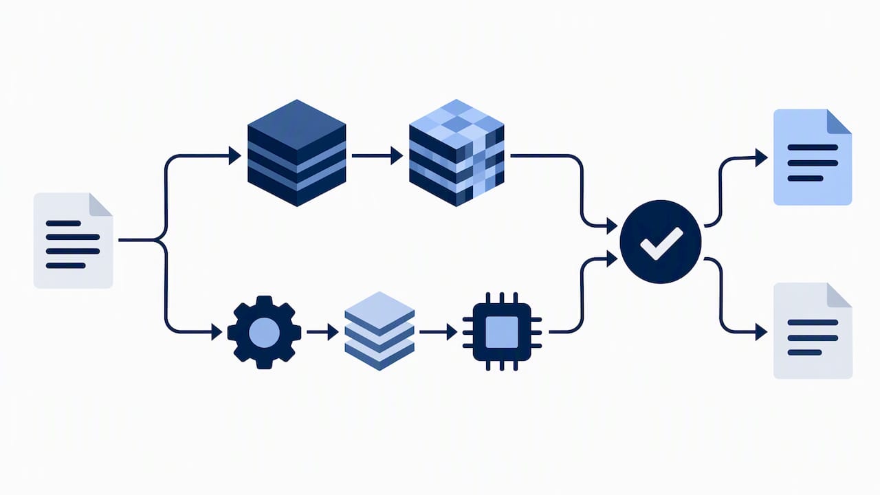
For numerical issues, check the obvious suspects first. Outlier channels, discussed earlier as the most common root cause of accuracy loss, can often be confirmed by inspecting activation statistics for the layers where outputs diverge. A mismatch between the calibration data distribution and the production prompt distribution is the second most common cause, and it is worth directly comparing a sample of calibration prompts against real production traffic when regressions appear only on certain input types.
For infrastructural issues, confirm that the runtime is actually using the optimized kernel path for your format and hardware rather than falling back to a slower emulation path, since a silent fallback can look like a performance regression rather than an outright failure. Library version mismatches between the quantization toolchain and the serving runtime are a frequent cause of this, which is why pinning versions alongside the checkpoint, as noted earlier, pays off directly here.
When regressions appear only in specific capabilities, structured output, long-context retrieval, domain terminology, treat that as a signal to add a targeted regression test for that capability going forward, rather than treating the single incident as resolved once the immediate symptom is patched.
Trade-offs we choose as systems integrators
We generally favor a smaller model at a higher bitwidth over a larger model pushed to the lowest bitwidth it can technically survive. A smaller, well-calibrated model is easier to validate, easier to roll back, and easier to explain to an auditor than a large model whose low-bit behavior depends on a method stacking multiple error-mitigation tricks.
For instruction-following and domain terminology, two of the most common regression points, we weight our evaluation suites more heavily toward the exact prompt patterns a client’s frontline teams will actually use rather than general benchmarks. A model that scores well on public instruction-following tests can still mishandle the specific terminology of a regulated industry, and that gap only shows up when you test for it directly.
On the operations side, this conservative posture scales better across an enterprise client base: a known, well-tested bitwidth and method combination is something we can support consistently, while chasing the lowest possible bit count model by model multiplies the number of edge cases a support team has to carry.
How Forge can help with quantized LLM deployments
We deploy and operate quantized LLMs inside infrastructure fully controlled by clients, utilizing webAI’s local-first platform into production. For organizations in regulated or high-security sectors, that means the calibration data, the checkpoints, and the model outputs never leave the environment we deploy into.

Our work on quantized deployments typically covers:
- Deployment of quantized models for local and air-gapped environments, including hardware and runtime matching considerations.
- Model integration and optimization, tuning bitwidth, method, and calibration to actual workloads rather than generic benchmarks.
- AI assistant rollout leveraging local AI Personas and capabilities, enabling frontline teams with fast, source-backed answers from large technical document libraries, fully offline.
- MLOps and runtime orchestration to maintain reproducible pipelines and auditable releases as models are updated over time.
Acting as the integrator rather than leaving a team to assemble a quantization pipeline from scratch helps reduce operational risk by embedding calibration versioning, regression testing, and rollback planning into managed rollouts. If a quantized deployment is on your roadmap, our solutions page outlines where to start, or you can review why organizations choose to work with us for sovereign AI.
FAQ
What is LLM model quantization?
LLM quantization reduces the numeric precision of a model’s weights, and sometimes its activations, from formats like FP32 or FP16 down to lower-bit formats such as INT8, INT4, or FP8. The main benefit is a smaller memory footprint, with throughput gains possible when the target hardware has native kernel support for the chosen format.
What is the best quantization method for LLMs?
There is no single best method: choice depends on model size, target hardware, and whether the workload is memory-bound or compute-bound. A 2025 PTQ taxonomy groups mainstream weight-only methods into compensation-based (GPTQ), optimization-based (OmniQuant), rotation-based (QuIP), and salience-based (AWQ) families, each suited to different deployment scenarios.
When should you quantize a model?
Quantize when memory or deployment cost is the binding constraint and you can validate the quantized model against your specific production prompts and capabilities, not just a perplexity score. Evaluation across model scales up to 405B parameters shows quantization behavior varies by model and method, so testing before rollout matters more than the bitwidth you pick.
How do I quantize a model?
Select your deployment target and workload type, choose a method and bitwidth that match it, assemble a versioned calibration dataset drawn from real production prompts, then run calibration through a toolchain like LLM Compressor or AutoFP8 for vLLM. Benchmark prefill and decode separately and run a full regression suite, not just perplexity, before releasing the checkpoint.
Does quantization always improve inference speed?
No. Quantization primarily reduces memory footprint, and speed gains depend on whether the target hardware has a native kernel for the chosen format. vLLM’s FP8 documentation reports throughput improvements for certain supported configurations, but unsupported hardware can fall back to slower emulation paths instead of running faster.
Sources
- Model quantization techniques — ROCm / AMD Quark
- A Comprehensive Evaluation of Quantized Instruction-Tuned Large Language Models
- FP8 — vLLM documentation
- MergeQuant: Accurate 4-bit Static Quantization of Large Language Models